MATLAB® Test Report
|
Timestamp: |
12-Jan-2026 16:11:16 |
|
Host: |
runnervmi13qx |
|
Platform: |
glnxa64 |
|
MATLAB Version: |
24.2.0.3070828 (R2024b) Update 7 |
|
Number of Tests: |
21 |
|
Testing Time: |
61.3931 seconds |
|
Overall Result: |
PASSED |

Overview
/home/runner/work/Applied-ODEs/Applied-ODEs/SoftwareTests/
|
28.6206 seconds |
||
|
|
||
|
32.7725 seconds |
||
|
|
||
Details
/home/runner/work/Applied-ODEs/Applied-ODEs/SoftwareTests/
SmokeTests
 SmokeRun
Class Setup Parameters: Project=matlab.project.Project
Test Parameters: File=CharacteristicEquations.mlx
SmokeRun
Class Setup Parameters: Project=matlab.project.Project
Test Parameters: File=CharacteristicEquations.mlx
The test passed. Duration: 18.9135 seconds
Events:
Diagnostic logged.
|
Timestamp: 12-Jan-2026 16:10:24 Verbosity: Terse Logged Diagnostic: Figure saved to: --> /tmp/156abed3-a3f6-4d69-824a-54521e325ac7/Figure_31e83713-be6b-4791-a1f4-aaeab39b5ffd.png
Event Location: SmokeTests[Project=matlab.project.Project]/SmokeRun(File=CharacteristicEquations.mlx) Stack: In /home/runner/work/Applied-ODEs/Applied-ODEs/SoftwareTests/SmokeTests.m (SmokeTests.SmokeRun) at 94 |
Diagnostic logged.
|
Timestamp: 12-Jan-2026 16:10:28 Verbosity: Terse Logged Diagnostic: Figure saved to: --> /tmp/156abed3-a3f6-4d69-824a-54521e325ac7/Figure_79c50571-42fd-4101-989f-9e0094ac2c5d.png
Event Location: SmokeTests[Project=matlab.project.Project]/SmokeRun(File=CharacteristicEquations.mlx) Stack: In /home/runner/work/Applied-ODEs/Applied-ODEs/SoftwareTests/SmokeTests.m (SmokeTests.SmokeRun) at 94 |
(Overview)
SmokeRun
Class Setup Parameters: Project=matlab.project.Project
Test Parameters: File=CheckYourWork.mlx
The test passed. Duration: 0.2063 seconds
(Overview)
SmokeRun
Class Setup Parameters: Project=matlab.project.Project
Test Parameters: File=Classification.mlx
The test passed. Duration: 0.1061 seconds
(Overview)
SmokeRun
Class Setup Parameters: Project=matlab.project.Project
Test Parameters: File=IntegratingFactors.mlx
The test passed. Duration: 2.7992 seconds
Event:
Diagnostic logged.
|
Timestamp: 12-Jan-2026 16:10:33 Verbosity: Terse Logged Diagnostic: Figure saved to: --> /tmp/156abed3-a3f6-4d69-824a-54521e325ac7/Figure_904ecb0b-81ea-4c30-9ac1-c6324afed0ea.png
Event Location: SmokeTests[Project=matlab.project.Project]/SmokeRun(File=IntegratingFactors.mlx) Stack: In /home/runner/work/Applied-ODEs/Applied-ODEs/SoftwareTests/SmokeTests.m (SmokeTests.SmokeRun) at 94 |
(Overview)
SmokeRun
Class Setup Parameters: Project=matlab.project.Project
Test Parameters: File=SeparationOfVariables.mlx
The test passed. Duration: 1.2919 seconds
Event:
Diagnostic logged.
|
Timestamp: 12-Jan-2026 16:10:35 Verbosity: Terse Logged Diagnostic: Figure saved to: --> /tmp/156abed3-a3f6-4d69-824a-54521e325ac7/Figure_c4e13475-6c04-495e-acae-b25658ba1720.png
Event Location: SmokeTests[Project=matlab.project.Project]/SmokeRun(File=SeparationOfVariables.mlx) Stack: In /home/runner/work/Applied-ODEs/Applied-ODEs/SoftwareTests/SmokeTests.m (SmokeTests.SmokeRun) at 94 |

(Overview)
SmokeRun
Class Setup Parameters: Project=matlab.project.Project
Test Parameters: File=SystemsOfODEs.mlx
The test passed. Duration: 1.9180 seconds
Event:
Diagnostic logged.
|
Timestamp: 12-Jan-2026 16:10:36 Verbosity: Terse Logged Diagnostic: Figure saved to: --> /tmp/156abed3-a3f6-4d69-824a-54521e325ac7/Figure_10835b30-bbe6-4f13-b2d5-d60f4be52185.png
Event Location: SmokeTests[Project=matlab.project.Project]/SmokeRun(File=SystemsOfODEs.mlx) Stack: In /home/runner/work/Applied-ODEs/Applied-ODEs/SoftwareTests/SmokeTests.m (SmokeTests.SmokeRun) at 94 |
(Overview)
SmokeRun
Class Setup Parameters: Project=matlab.project.Project
Test Parameters: File=UndeterminedCoefficients.mlx
The test passed. Duration: 3.3857 seconds
Events:
Diagnostic logged.
|
Timestamp: 12-Jan-2026 16:10:39 Verbosity: Terse Logged Diagnostic: Figure saved to: --> /tmp/156abed3-a3f6-4d69-824a-54521e325ac7/Figure_2fbc4b01-985d-4d0a-8132-a5039d7e0814.png
Event Location: SmokeTests[Project=matlab.project.Project]/SmokeRun(File=UndeterminedCoefficients.mlx) Stack: In /home/runner/work/Applied-ODEs/Applied-ODEs/SoftwareTests/SmokeTests.m (SmokeTests.SmokeRun) at 94 |
Diagnostic logged.
|
Timestamp: 12-Jan-2026 16:10:40 Verbosity: Terse Logged Diagnostic: Figure saved to: --> /tmp/156abed3-a3f6-4d69-824a-54521e325ac7/Figure_4dd8464d-0cc0-4d6d-8770-a9aabc50d004.png
Event Location: SmokeTests[Project=matlab.project.Project]/SmokeRun(File=UndeterminedCoefficients.mlx) Stack: In /home/runner/work/Applied-ODEs/Applied-ODEs/SoftwareTests/SmokeTests.m (SmokeTests.SmokeRun) at 94 |
(Overview)
SolnSmokeTests
ExistSolns
Class Setup Parameters: Project=matlab.project.Project
Test Parameters: File=CharacteristicEquations.mlx
The test passed. Duration: 0.0650 seconds
(Overview)
ExistSolns
Class Setup Parameters: Project=matlab.project.Project
Test Parameters: File=CheckYourWork.mlx
The test passed. Duration: 0.0058 seconds
(Overview)
ExistSolns
Class Setup Parameters: Project=matlab.project.Project
Test Parameters: File=Classification.mlx
The test passed. Duration: 0.0053 seconds
(Overview)
ExistSolns
Class Setup Parameters: Project=matlab.project.Project
Test Parameters: File=IntegratingFactors.mlx
The test passed. Duration: 0.0052 seconds
(Overview)
ExistSolns
Class Setup Parameters: Project=matlab.project.Project
Test Parameters: File=SeparationOfVariables.mlx
The test passed. Duration: 0.0076 seconds
(Overview)
ExistSolns
Class Setup Parameters: Project=matlab.project.Project
Test Parameters: File=SystemsOfODEs.mlx
The test passed. Duration: 0.0047 seconds
(Overview)
ExistSolns
Class Setup Parameters: Project=matlab.project.Project
Test Parameters: File=UndeterminedCoefficients.mlx
The test passed. Duration: 0.0047 seconds
(Overview)
SmokeRun
Class Setup Parameters: Project=matlab.project.Project
Test Parameters: File=CharacteristicEquations.mlx
The test passed. Duration: 8.9491 seconds
Events:
Diagnostic logged.
|
Timestamp: 12-Jan-2026 16:10:48 Verbosity: Terse Logged Diagnostic: Figure saved to: --> /tmp/156abed3-a3f6-4d69-824a-54521e325ac7/Figure_c04d4f5c-9159-4f24-a425-dc11146d32f5.png
Event Location: SolnSmokeTests[Project=matlab.project.Project]/SmokeRun(File=CharacteristicEquations.mlx) Stack: In /home/runner/work/Applied-ODEs/Applied-ODEs/SoftwareTests/SolnSmokeTests.m (SolnSmokeTests.SmokeRun) at 110 |
Diagnostic logged.
|
Timestamp: 12-Jan-2026 16:10:49 Verbosity: Terse Logged Diagnostic: Figure saved to: --> /tmp/156abed3-a3f6-4d69-824a-54521e325ac7/Figure_6c62b0c9-8dc5-40e7-9e1e-d8c85979648e.png
Event Location: SolnSmokeTests[Project=matlab.project.Project]/SmokeRun(File=CharacteristicEquations.mlx) Stack: In /home/runner/work/Applied-ODEs/Applied-ODEs/SoftwareTests/SolnSmokeTests.m (SolnSmokeTests.SmokeRun) at 110 |
(Overview)
SmokeRun
Class Setup Parameters: Project=matlab.project.Project
Test Parameters: File=CheckYourWork.mlx
The test passed. Duration: 1.6219 seconds
Event:
Diagnostic logged.
|
Timestamp: 12-Jan-2026 16:10:51 Verbosity: Terse Logged Diagnostic: Figure saved to: --> /tmp/156abed3-a3f6-4d69-824a-54521e325ac7/Figure_3ce7ec74-f871-4743-a381-ca51c11238c4.png
Event Location: SolnSmokeTests[Project=matlab.project.Project]/SmokeRun(File=CheckYourWork.mlx) Stack: In /home/runner/work/Applied-ODEs/Applied-ODEs/SoftwareTests/SolnSmokeTests.m (SolnSmokeTests.SmokeRun) at 110 |
(Overview)
SmokeRun
Class Setup Parameters: Project=matlab.project.Project
Test Parameters: File=Classification.mlx
The test passed. Duration: 0.0793 seconds
(Overview)
SmokeRun
Class Setup Parameters: Project=matlab.project.Project
Test Parameters: File=IntegratingFactors.mlx
The test passed. Duration: 1.1355 seconds
Event:
Diagnostic logged.
|
Timestamp: 12-Jan-2026 16:10:52 Verbosity: Terse Logged Diagnostic: Figure saved to: --> /tmp/156abed3-a3f6-4d69-824a-54521e325ac7/Figure_0931ec65-66d6-4fbd-8ebd-3b3aa4eb2dcf.png
Event Location: SolnSmokeTests[Project=matlab.project.Project]/SmokeRun(File=IntegratingFactors.mlx) Stack: In /home/runner/work/Applied-ODEs/Applied-ODEs/SoftwareTests/SolnSmokeTests.m (SolnSmokeTests.SmokeRun) at 110 |

(Overview)
SmokeRun
Class Setup Parameters: Project=matlab.project.Project
Test Parameters: File=SeparationOfVariables.mlx
The test passed. Duration: 0.8664 seconds
Event:
Diagnostic logged.
|
Timestamp: 12-Jan-2026 16:10:53 Verbosity: Terse Logged Diagnostic: Figure saved to: --> /tmp/156abed3-a3f6-4d69-824a-54521e325ac7/Figure_36cdcd76-cd87-4bb1-95dd-60fab75de4ce.png
Event Location: SolnSmokeTests[Project=matlab.project.Project]/SmokeRun(File=SeparationOfVariables.mlx) Stack: In /home/runner/work/Applied-ODEs/Applied-ODEs/SoftwareTests/SolnSmokeTests.m (SolnSmokeTests.SmokeRun) at 110 |

(Overview)
SmokeRun
Class Setup Parameters: Project=matlab.project.Project
Test Parameters: File=SystemsOfODEs.mlx
The test passed. Duration: 12.5519 seconds
Event:
Diagnostic logged.
|
Timestamp: 12-Jan-2026 16:11:06 Verbosity: Terse Logged Diagnostic: Figure saved to: --> /tmp/156abed3-a3f6-4d69-824a-54521e325ac7/Figure_4738d154-0b91-474d-a2fa-b42353798f39.png
Event Location: SolnSmokeTests[Project=matlab.project.Project]/SmokeRun(File=SystemsOfODEs.mlx) Stack: In /home/runner/work/Applied-ODEs/Applied-ODEs/SoftwareTests/SolnSmokeTests.m (SolnSmokeTests.SmokeRun) at 110 |
(Overview)
SmokeRun
Class Setup Parameters: Project=matlab.project.Project
Test Parameters: File=UndeterminedCoefficients.mlx
The test passed. Duration: 7.4700 seconds
Events:
Diagnostic logged.
|
Timestamp: 12-Jan-2026 16:11:12 Verbosity: Terse Logged Diagnostic: Figure saved to: --> /tmp/156abed3-a3f6-4d69-824a-54521e325ac7/Figure_c990a676-88fa-4e85-bb43-7e1a4eb52460.png
Event Location: SolnSmokeTests[Project=matlab.project.Project]/SmokeRun(File=UndeterminedCoefficients.mlx) Stack: In /home/runner/work/Applied-ODEs/Applied-ODEs/SoftwareTests/SolnSmokeTests.m (SolnSmokeTests.SmokeRun) at 110 |
Diagnostic logged.
|
Timestamp: 12-Jan-2026 16:11:13 Verbosity: Terse Logged Diagnostic: Figure saved to: --> /tmp/156abed3-a3f6-4d69-824a-54521e325ac7/Figure_f89b4057-a993-4b57-967f-d9fccc71ff41.png
Event Location: SolnSmokeTests[Project=matlab.project.Project]/SmokeRun(File=UndeterminedCoefficients.mlx) Stack: In /home/runner/work/Applied-ODEs/Applied-ODEs/SoftwareTests/SolnSmokeTests.m (SolnSmokeTests.SmokeRun) at 110 |
(Overview)
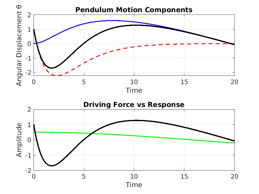
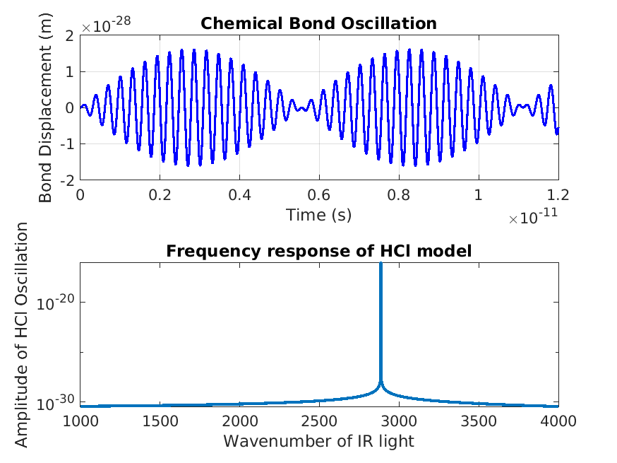
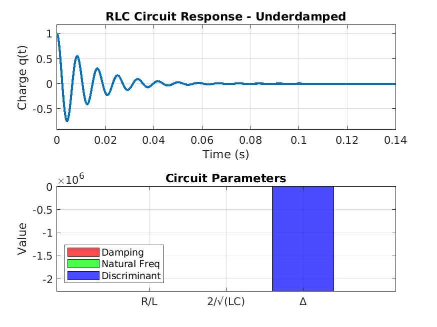
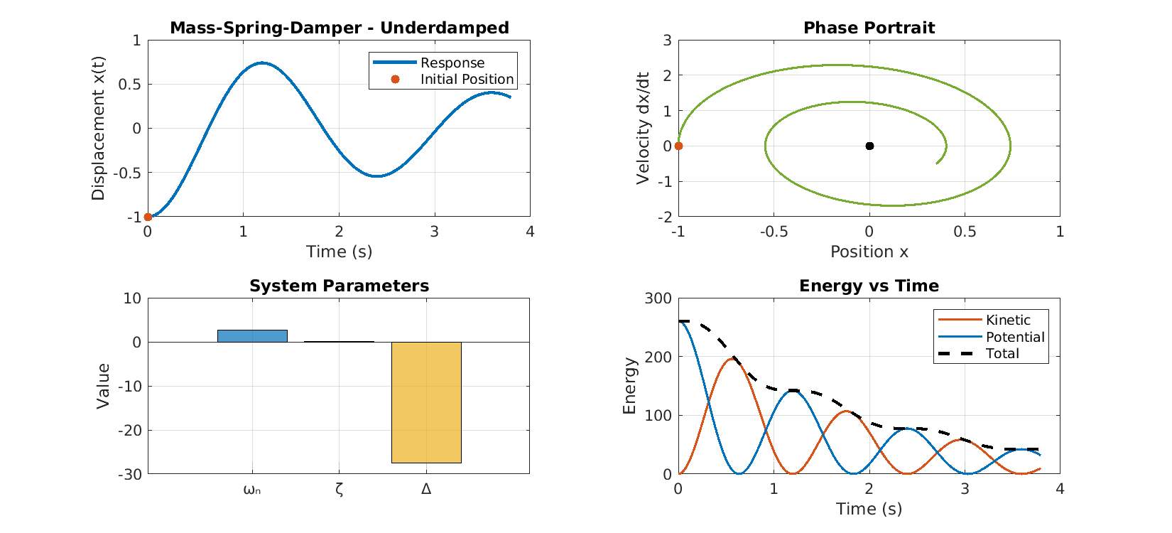
Command Window Text
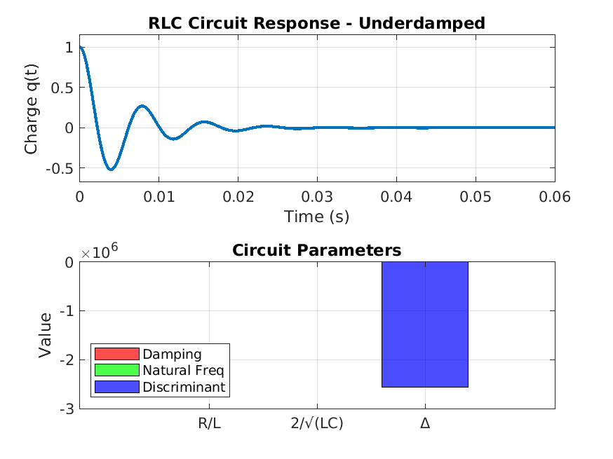
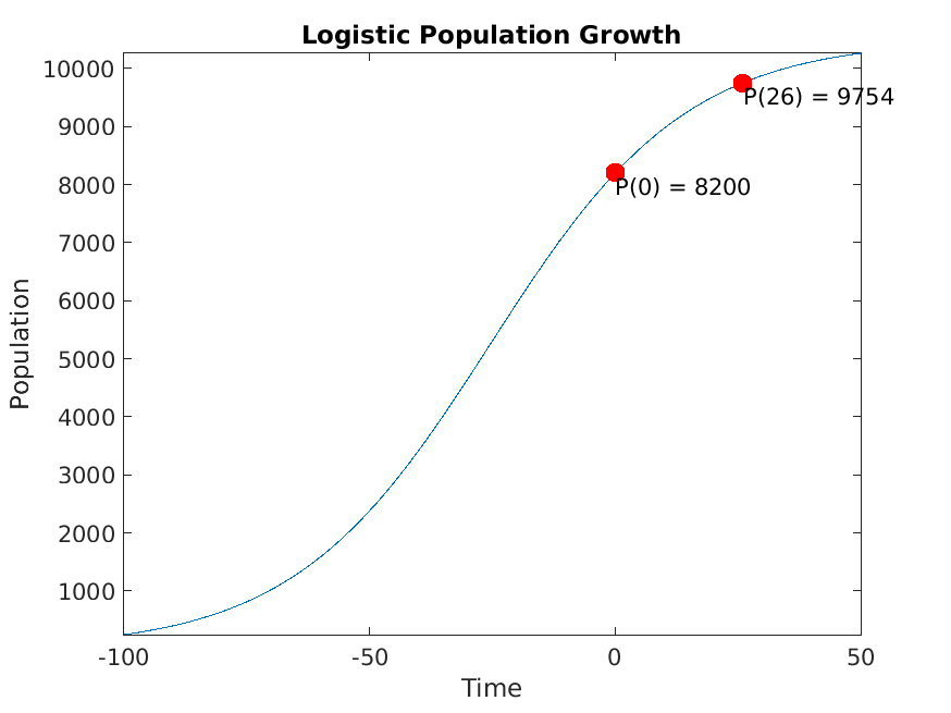
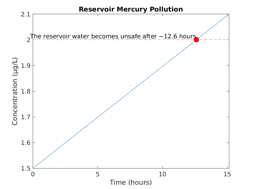
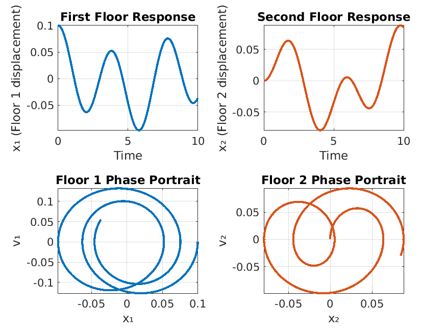
Running SmokeTests >> Running CharacteristicEquations.mlx Solve 12*y(x) - 7*diff(y(x), x) + diff(y(x), x, x) == 0 This is the default solution. The characteristic polynomial of a second order linear ODE will be quadratic. This is the default. Please compute and enter the roots of the characteristic polynomial. This is the default solution. Solve y(x) - 2*diff(y(x), x) + diff(y(x), x, x) == 0 This is the default solution. The characteristic polynomial of a second order linear ODE will be quadratic. This is the default. Please compute and enter the roots of the characteristic polynomial. This is the default solution. Solve 5*y(x) - diff(y(x), x) + 5*diff(y(x), x, x) == 0 This is the default solution. The characteristic polynomial of a second order linear ODE will be quadratic. This is the default. Please compute and enter the roots of the characteristic polynomial. This is the default solution. Solve 50*y(x) + 20*diff(y(x), x) + 2*diff(y(x), x, x) == 0 This is the default solution. The characteristic polynomial of a second order linear ODE will be quadratic. This is the default. Please compute and enter the roots of the characteristic polynomial. This is the default value. Once you generate a problem, there will certainly be known roots. This is the default solution. [Terse] Diagnostic logged (2026-01-12 16:10:24): Figure saved to: --> /tmp/156abed3-a3f6-4d69-824a-54521e325ac7/Figure_31e83713-be6b-4791-a1f4-aaeab39b5ffd.png [Terse] Diagnostic logged (2026-01-12 16:10:28): Figure saved to: --> /tmp/156abed3-a3f6-4d69-824a-54521e325ac7/Figure_79c50571-42fd-4101-989f-9e0094ac2c5d.png .>> Running CheckYourWork.mlx .>> Running Classification.mlx Please select one or more variables. Please select an answer. Please select one or more variables. Please select an answer. Please enter a nonzero order. Please select an answer. Please select an answer. Please enter a nonzero order. Please select an answer. Please select an answer. Please enter a nonzero order. Please select an answer. Please select an answer. .>> Running IntegratingFactors.mlx Please enter a nonzero expression. Please enter a nonzero expression. Please enter a nonzero expression. Please enter a nonzero expression. Please enter a nonzero expression. Please enter a nonzero expression. Please enter a nonzero expression. Please enter a nonzero expression. Please enter a nonzero expression. Please enter a nonzero expression. Please enter a nonzero expression. Please enter a positive integer. We start with our generic formula for chemical concentration: diff(M(t), t) == concentrationIn*rateIn - (rateOut*M(t))/(volInit + t*(rateIn - rateOut)) Plugging in the parameters, we have: diff(M(t), t) == 4 - M(t)/(50*(t/50 + 100)) [Terse] Diagnostic logged (2026-01-12 16:10:33): Figure saved to: --> /tmp/156abed3-a3f6-4d69-824a-54521e325ac7/Figure_904ecb0b-81ea-4c30-9ac1-c6324afed0ea.png .>> Running SeparationOfVariables.mlx Please select an answer. Please select an answer. Please select an answer. Please enter a nonzero expression. Please enter a nonzero expression. Please enter a nonzero expression. Please enter a nonzero expression. Please enter a nonzero expression. Please enter a nonzero expression. Please enter a nonzero expression. Please enter a nonzero expression. Please enter a positive integer. Please enter a nonzero expression. Please enter a nonzero expression. Please enter a nonzero expression. P(t) == (P0*k*exp(r*t))/((k - P0) + P0*exp(r*t)) Plugging in these custom parameters, we get: P(t) == (86100000*exp(t/20))/(8200*exp(t/20) + 2300) Here's a plot of the solution: [Terse] Diagnostic logged (2026-01-12 16:10:35): Figure saved to: --> /tmp/156abed3-a3f6-4d69-824a-54521e325ac7/Figure_c4e13475-6c04-495e-acae-b25658ba1720.png .>> Running SystemsOfODEs.mlx Consider the following system of differential equations dx/dt == 3*x + y dy/dt == 3*x + 2*y This is the default. Please enter a non-zero matrix. Please enter the eigenvalues of A. Incorrect. Solve the equation (A - lambda*I)*v == 0 Incorrect. Solve the equation (A - lambda*I)*v == 0 Let beta == 0.2 and gamma == 0.15. Incorrect. In this case, A should be a 2x2 matrix. Please enter the eigenvalues of A. You can be more precise than this. Please select a different answer. Basic reproduction number R₀ = 2 R₀ > 1: Epidemic will occur This is the default. Please enter the correct matrix. This is the default. Please enter the computed eigenvalues. [Terse] Diagnostic logged (2026-01-12 16:10:36): Figure saved to: --> /tmp/156abed3-a3f6-4d69-824a-54521e325ac7/Figure_10835b30-bbe6-4f13-b2d5-d60f4be52185.png .>> Running UndeterminedCoefficients.mlx The proposed solution is y == (2*x)/9 + C2*exp(x) + x^2/3 + C1*exp(3*x) + 38/27. Plugging into the original ODE we have - 2*x + x^2 + 4 == - 2*x + x^2 + 4, which is true! Solve - 192*y(x) + 3*diff(y(x), x, x) == - 4*x - 5*x^2 - 2*x^3 - 5*x^4 + 4 This is the default. Please enter a solution and resubmit. This is the default. Please enter a solution and resubmit. This is the default. Please enter a solution and resubmit. This is the default, please enter a proposed solution. Solve 9*y(x) + 6*diff(y(x), x) + diff(y(x), x, x) == -2*exp(2*x) This is the default. Please enter a solution and resubmit. This is the default. Please enter a solution and resubmit. ans = logical 0 This is the default. Please enter a solution and resubmit. ans = logical 0 Solve 5*y(x) - 3*diff(y(x), x) + diff(y(x), x, x) == 2*cos(4*x) This is the default. Please enter a solution and resubmit. This is the default. Please enter a solution and resubmit. ans = logical 0 This is the default. Please enter a solution and resubmit. ans = logical 0 Solve 17*y(x) - 8*diff(y(x), x) + diff(y(x), x, x) == -2*cos(4*x)*exp(x) This is the default. Please enter a solution and resubmit. This is the default. Please enter a solution and resubmit. ans = logical 0 This is the default. Please enter a solution and resubmit. ans = logical 0 This is the default value. The solution is not just the forcing function. Parameters: γ=1.00, ω₀=0.50, F₀=0.50, ω=0.10 -(exp(-t/2)*(7*t - 2))/2 This is the default. The spring constant is not 0. Bond wavenumber: 2886, External wavenumber: 2880, Response Amplitude: 8.1353e-29 [Terse] Diagnostic logged (2026-01-12 16:10:39): Figure saved to: --> /tmp/156abed3-a3f6-4d69-824a-54521e325ac7/Figure_2fbc4b01-985d-4d0a-8132-a5039d7e0814.png [Terse] Diagnostic logged (2026-01-12 16:10:40): Figure saved to: --> /tmp/156abed3-a3f6-4d69-824a-54521e325ac7/Figure_4dd8464d-0cc0-4d6d-8770-a9aabc50d004.png . Done SmokeTests __________ Running SolnSmokeTests .......>> Running CharacteristicEquationsSoln.mlx Solve 15*y(x) - 8*diff(y(x), x) + diff(y(x), x, x) == 0 Correct! The characteristic polynomial is: - 8*x + x^2 + 15 == 0 Correct! The roots are r_1 == 3, and r_2 == 5. Correct! The solution is: y(x) == C1*exp(3*x) + C2*exp(5*x) Solve diff(y(x), x, x) == 0 Correct! The characteristic polynomial is: x^2 == 0 Correct! The solution is r == 0 twice! Correct! The solution is: y(x) == C2 + C1*x Solve - 2*y(x) + 3*diff(y(x), x) - 4*diff(y(x), x, x) == 0 Correct! The characteristic polynomial is: 3*x - 4*x^2 - 2 == 0 Correct! The roots are r_1 == - (23^(1/2)*1i)/8 + 3/8, and r_2 == (23^(1/2)*1i)/8 + 3/8. Correct! The solution is: y(x) == C1*exp((3*x)/8)*cos((23^(1/2)*x)/8) - C2*exp((3*x)/8)*sin((23^(1/2)*x)/8) Solve 27*y(x) + 18*diff(y(x), x) + 3*diff(y(x), x, x) == 0 Correct! The characteristic polynomial is: 18*x + 3*x^2 + 27 == 0 Correct! The solution is r == -3 twice! Correct, this problem has repeated roots. Correct! The solution is: y(x) == C1*exp(-3*x) + C2*x*exp(-3*x) --- RLC Circuit Analysis --- L = 3.50 H, R = 0.50 kΩ = 500 Ω , C = 0.500 µF = 5.00 * 1e-7 F Characteristic equation: r² + 142.857r + 571428.571 = 0 Damping: 142.857 Natural frequency: 1511.858 Discriminant: -2265306.122 System type: Underdamped Complex roots: r = -71.429 ± 752.547i Assume q(0)=1 and q'(0)=0. Differential equation solution: q(t) = (exp(-(500*t)/7)*(79456894976000007*cos((3*52971263317333338^(1/2)*t)/917504) + 32768000*52971263317333338^(1/2)*sin((3*52971263317333338^(1/2)*t)/917504)))/79456894976000007 --- Mass-Spring-Damper Analysis --- m = 75.00 kg, c = 38.00 N·s/m, k = 521.00 N/m Initial conditions: x₀ = -1.00 m, v₀ = 0.00 m/s Natural frequency: ωₙ = 2.636 rad/s Damping ratio: ζ = 0.096 Discriminant: -27.530 System type: Underdamped Complex roots: r = -0.253 ± 2.623i Damped frequency: ωd = 2.623 rad/s Differential equation solution: x(t) = -(exp(-(19*t)/75)*(38714*cos((38714^(1/2)*t)/75) + 19*38714^(1/2)*sin((38714^(1/2)*t)/75)))/38714 [Terse] Diagnostic logged (2026-01-12 16:10:48): Figure saved to: --> /tmp/156abed3-a3f6-4d69-824a-54521e325ac7/Figure_c04d4f5c-9159-4f24-a425-dc11146d32f5.png [Terse] Diagnostic logged (2026-01-12 16:10:49): Figure saved to: --> /tmp/156abed3-a3f6-4d69-824a-54521e325ac7/Figure_6c62b0c9-8dc5-40e7-9e1e-d8c85979648e.png .>> Running CheckYourWorkSoln.mlx MyGeneralSolution = (35*t)/18 + (7*t^2)/6 + C1*exp(2*t) + C2*exp(3*t) + 97/108 MySolution = (35*t)/18 + (37*exp(2*t))/4 - (193*exp(3*t))/27 + (7*t^2)/6 + 97/108 MyUnexpectedSolution = C1*airy(0, t) + C2*airy(2, t) MyNonSolution = C1 + int(exp(-t^3), t, 'IgnoreSpecialCases', true, 'IgnoreAnalyticConstraints', true) QuadraticEquation = a*x^2 + b*x + c == 0 Roots = -(b + (b^2 - 4*a*c)^(1/2))/(2*a) -(b - (b^2 - 4*a*c)^(1/2))/(2*a) My differential equation is: 6*x(t) - 5*diff(x(t), t) + diff(x(t), t, t) == 7*t^2 - 2 and the general solution is: (35*t)/18 + (37*exp(2*t))/4 - (193*exp(3*t))/27 + (7*t^2)/6 + 97/108 [Terse] Diagnostic logged (2026-01-12 16:10:51): Figure saved to: --> /tmp/156abed3-a3f6-4d69-824a-54521e325ac7/Figure_3ce7ec74-f871-4743-a381-ca51c11238c4.png .>> Running ClassificationSoln.mlx Correct! b and c are the independent variables in this equation. Correct! This is a partial differential equation, because it has more than one independent variable. Correct! b is the only independent variable in this equation. Correct! This is an ordinary differential equation, because it has one independent variable. Correct! The fourth derivative of y is the highest derivative that appears in the equation, so the order is 4. Correct! All coefficients of y and its derivatatives are constant or functions of t, so the equation is linear. Correct! The trivial solution y=0 is not a solution, so the equation is nonhomogeneous. Correct! The third derivative of y is the highest derivative that appears in the equation, so the order is 3. Correct! The equation has a nonlinear term y' * y, so the equation is nonlinear. Correct! Because the equation is nonlinear, we can't assess its homogeneity. Correct! The second derivative of y is the highest derivative that appears in the equation, so the order is 2. Correct! All coefficients of y and its derivatatives are constant or functions of t, so the equation is linear. Correct! The trivial solution y=0 is a solution, so the equation is homogeneous. . >> Running IntegratingFactorsSoln.mlx Correct! See below for a detailed explanation. Correct! See below for a detailed explanation. Correct! See below for a detailed explanation. Correct! See below for a detailed explanation. Correct! See below for a detailed explanation. Correct! See below for a detailed explanation. Correct! See below for a detailed explanation. Correct! See below for a detailed explanation. Correct! See below for a detailed explanation. Correct! See below for a detailed explanation. Correct! See below for a detailed explanation. Starting with the equation from part (c): M == (20000*t + 2*t^2 + C)/(5000 + t) Remember that M represents the *quantity* of mercury in the water, so we have M(0) = 1.5 * 100 = 150. Solve for C, plugging in M = 150 and t = 0: 150 == (0 + 0 + C)/(5000 + 0) 150 == C/5000 C == 750000 Finally, plugging this value for C back into the equation from part (c), we get: M == (20000*t + 2*t^2 + 750000)/(5000 + t) Correct! See below for a detailed explanation. We start with our generic formula for chemical concentration: diff(M(t), t) == concentrationIn*rateIn - (rateOut*M(t))/(volInit + t*(rateIn - rateOut)) Plugging in the parameters, we have: diff(M(t), t) == 4 - M(t)/(50*(t/50 + 100)) [Terse] Diagnostic logged (2026-01-12 16:10:52): Figure saved to: --> /tmp/156abed3-a3f6-4d69-824a-54521e325ac7/Figure_0931ec65-66d6-4fbd-8ebd-3b3aa4eb2dcf.png .>> Running SeparationOfVariablesSoln.mlx Correct! This can be rewritten as: (1/y)*dy == 3*x^2*dx Correct! Using y' = dy/dx, this can be rewritten as: (1/y^2)*dy == (e^x/x)*dx Correct! There is no way to separate the x and y terms in this equation, so it is not separable. Correct! See below for a detailed explanation. Correct! See below for a detailed explanation. Correct! See below for a detailed explanation. Correct! See below for a detailed explanation. Correct! See below for a detailed explanation. Correct! See below for a detailed explanation. Correct! See below for a detailed explanation. Correct! See below for a detailed explanation. Correct! See below for a detailed explanation. Correct! See below for a detailed explanation. Correct! See below for a detailed explanation. Correct! See below for a detailed explanation. P(t) == (P0*k*exp(r*t))/((k - P0) + P0*exp(r*t)) Plugging in these custom parameters, we get: P(t) == (86100000*exp(t/20))/(8200*exp(t/20) + 2300) Here's a plot of the solution: [Terse] Diagnostic logged (2026-01-12 16:10:53): Figure saved to: --> /tmp/156abed3-a3f6-4d69-824a-54521e325ac7/Figure_36cdcd76-cd87-4bb1-95dd-60fab75de4ce.png .>> Running SystemsOfODEsSoln.mlx Consider the following system of differential equations dx/dt == - x - 3*y dy/dt == - 5*x + 5*y Correct! The system dx/dt == - x - 3*y dy/dt == - 5*x + 5*y can be written as: matrix([[dx/dt], [dy/dt]]) == matrix([[-1, -3], [-5, 5]])*matrix([[x], [y]]) So A == matrix([[-1, -3], [-5, 5]]) Correct! To find eigenvalues, solve det(A - lambda*I) == 0: det(matrix([[- lambda - 1, -3], [-5, - lambda + 5]])) == 0 - 4*lambda + lambda^2 - 20 == 0 lambda_1 == (4 + sqrt((-4)^2 - (-80)))/2, lambda_1 == 2*6^(1/2) + 2 lambda_2 == (4 - sqrt((-4)^2 - (-80)))/2, lambda_2 == - 2*6^(1/2) + 2 For lambda == 2*6^(1/2) + 2, solve (A - lambda*I)*v == 0 matrix([[- 2*6^(1/2) - 3, -3], [-5, - 2*6^(1/2) + 3]])*matrix([[v_1], [v_2]]) == matrix([[0], [0]]) matrix([[v_1], [v_2]]) == matrix([[- (2*6^(1/2))/5 + 3/5], [1]]) For lambda == - 2*6^(1/2) + 2, solve (A - lambda*I)*v == 0 matrix([[2*6^(1/2) - 3, -3], [-5, 2*6^(1/2) + 3]])*matrix([[v_1], [v_2]]) == matrix([[0], [0]]) matrix([[v_1], [v_2]]) == matrix([[(2*6^(1/2))/5 + 3/5], [1]]) x(t) == c_1*exp(-t*(2*6^(1/2) - 2))*((2*6^(1/2))/5 + 3/5) - c_2*exp(t*(2*6^(1/2) + 2))*((2*6^(1/2))/5 - 3/5) y(t) == c_1*exp(-t*(2*6^(1/2) - 2)) + c_2*exp(t*(2*6^(1/2) + 2)) Checking... matrix([[- c_1*exp(-t*(2*6^(1/2) - 2))*(2*6^(1/2) - 2)*((2*6^(1/2))/5 + 3/5) - c_2*exp(t*(2*6^(1/2) + 2))*(2*6^(1/2) + 2)*((2*6^(1/2))/5 - 3/5)], [c_2*exp(t*(2*6^(1/2) + 2))*(2*6^(1/2) + 2) - c_1*exp(-2*t*(6^(1/2) - 1))*(2*6^(1/2) - 2)]]) - matrix([[-1, -3], [-5, 5]])*matrix([[c_1*exp(-t*(2*6^(1/2) - 2))*((2*6^(1/2))/5 + 3/5) - c_2*exp(t*(2*6^(1/2) + 2))*((2*6^(1/2))/5 - 3/5)], [c_1*exp(-t*(2*6^(1/2) - 2)) + c_2*exp(t*(2*6^(1/2) + 2))]]) == matrix([[0], [0]]) Let beta == 0.2 and gamma == 0.17. Plugging in the values for beta == 0.2 and gamma == 0.17 we see that we get: Correct! The system dS/dt == -0.2*I dI/dt == 0.03*I which can be written as matrix([[dS/dt], [dI/dt]]) == matrix([[0, -0.2], [0, 0.03]])*matrix([[S], [I]]) So A == matrix([[0, -0.2], [0, 0.03]]) Correct! To find eigenvalues, solve det(A - lambda*I) == 0: det(matrix([[-1.0*lambda, -0.2], [0, - 1.0*lambda + 0.03]])) == 0 (lambda*(100*lambda - 3))/100 == 0 lambda_1 == (0.03 + sqrt((-0.03)^2 - 0.0))/2.0, lambda_1 == 0.03 lambda_2 == (0.03 - sqrt((-0.03)^2 - 0.0))/2.0, lambda_2 == 0.0 Not quite. What do positive eigenvalues mean for the long-term growth of solutions? Basic reproduction number R₀ = 1 The disease is endemic in the population. Correct! The coefficient matrix represents the building dynamics. A == matrix([[0, 1, 0, 0], [-2*omega^2, 0, omega^2, 0], [0, 0, 0, 1], [omega^2, 0, -omega^2, 0]]) dx_1/dt == v_1 dv_1/dt == - 2*omega^2*x_1 + omega^2*x_2 dx_2/dt == v_2 dv_2/dt == omega^2*x_1 - omega^2*x_2 Correct! The eigenvalues are ±(- 5^(1/2)/2 - 3/2)^(1/2) and ±(5^(1/2)/2 - 3/2)^(1/2), or approximately ±1.618i and ±0.618i, representing the natural frequencies of the building modes. The characteristic equation is: lambda^4 + 3*lambda^2 + 1 == 0 [Terse] Diagnostic logged (2026-01-12 16:11:06): Figure saved to: --> /tmp/156abed3-a3f6-4d69-824a-54521e325ac7/Figure_4738d154-0b91-474d-a2fa-b42353798f39.png .>> Running UndeterminedCoefficientsSoln.mlx The proposed solution is y == (2*x)/9 + C2*exp(x) + x^2/3 + C1*exp(3*x) + 38/27. Plugging into the original ODE we have - 2*x + x^2 + 4 == - 2*x + x^2 + 4, which is true! Solve - 5*y(x) + 4*diff(y(x), x) - diff(y(x), x, x) == - x - 5*x^2 + 5*x^3 + x^4 - 4 WorkOutGuess = A*x^4 + B*x^3 + C*x^2 + D*x + E Correct! The guess is y_p == E + D*x + A*x^4 + B*x^3 + C*x^2 Correct! y_p == - (1101*x)/625 - (307*x^2)/125 - (41*x^3)/25 - x^4/5 + 1166/3125 Correct! The solution is: y(x) == C1*exp(2*x)*cos(x) - C2*exp(2*x)*sin(x) That is correct! The general solution is y == - (1101*x)/625 - (307*x^2)/125 - (41*x^3)/25 - x^4/5 + C1*exp(2*x)*cos(x) - C2*exp(2*x)*sin(x) + 1166/3125 Solve y(x) - 2*diff(y(x), x) + diff(y(x), x, x) == 3*exp(-x) WorkOutGuess2 = A*exp(-x) Correct! The guess is y_p == A*exp(-x) Correct! y_p == (3*exp(-x))/4 ans = logical 1 Correct! The solution is: y(x) == C1*exp(x) + C2*x*exp(x) ans = logical 1 Solve 20*y(x) - 9*diff(y(x), x) + diff(y(x), x, x) == -2*cos(x) WorkOutGuess3 = B*cos(x) + A*sin(x) Correct! The guess is y_p == B*cos(x) + A*sin(x) Correct! y_p == -(442^(1/2)*cos(x + atan(9/19)))/221 ans = logical 1 Correct! The solution is: y(x) == C1*exp(4*x) + C2*exp(5*x) ans = logical 1 Solve 32*y(x) + 8*diff(y(x), x) + diff(y(x), x, x) == exp(-4*x)*(3*x^3*cos(4*x) + 4*x^4*sin(4*x)) WorkOutGuess4 = x*exp(-4*x)*(cos(4*x)*(A*x^4 + B*x^3 + C*x^2 + D*x + E) - sin(4*x)*(F*x^4 + G*x^3 + H*x^2 + I*x + J)) Technically correct! Conventionally, this guess is written with positive coefficients as y_p == x*exp(-4*x)*(cos(4*x)*(E + D*x + A*x^4 + B*x^3 + C*x^2) + sin(4*x)*(J + I*x + F*x^4 + G*x^3 + H*x^2)) Please try again. ans = logical 0 Correct! The solution is: y(x) == C1*cos(4*x)*exp(-4*x) - C2*sin(4*x)*exp(-4*x) ans = logical 1 Correct! The steady-state solution is x_p(t) == (F_0*t*sin(omega*t))/(2*(k*m)^(1/2)). Parameters: γ=0.22, ω₀=1.80, F₀=0.50, ω=3.60 -(3*exp(-(11*t)/100)*(2483*cos((13*191^(1/2)*t)/100) + 11*191^(1/2)*sin((13*191^(1/2)*t)/100)))/24830 Correct! The computed value for the spring coefficient for HCl is approximately 476 N/m. Bond wavenumber: 2886, External wavenumber: 2886, Response Amplitude: 1.8382e-15 [Terse] Diagnostic logged (2026-01-12 16:11:12): Figure saved to: --> /tmp/156abed3-a3f6-4d69-824a-54521e325ac7/Figure_c990a676-88fa-4e85-bb43-7e1a4eb52460.png [Terse] Diagnostic logged (2026-01-12 16:11:13): Figure saved to: --> /tmp/156abed3-a3f6-4d69-824a-54521e325ac7/Figure_f89b4057-a993-4b57-967f-d9fccc71ff41.png . Done SolnSmokeTests __________